Detailed guide to setting priors
James Uanhoro
priors.RmdDefault priors
We begin by loading the package:
## ## ################################################################################# This is minorbsem 0.2.16.9001##
## All users of R (or SEM) are invited to report bugs, submit functions or ideas
## for functions. An efficient way to do this is to open an issue on GitHub
## https://github.com/jamesuanhoro/minorbsem/issues/.## ###############################################################################The default priors are:
priors_default <- new_mbsempriors()
priors_default
## An object of class "mbsempriors"
## Slot "lkj_shape":
## [1] 2
##
## Slot "ml_par":
## [1] 0
##
## Slot "sl_par":
## [1] 1
##
## Slot "rs_par":
## [1] 1
##
## Slot "rc_par":
## [1] 2
##
## Slot "sc_par":
## [1] 0.5
##
## Slot "rm_par":
## [1] 0.15
lkj_shape
The lkj_shape parameter is for setting priors on the
interfactor correlation matrix. By default this value is 2, and implies
each correlation in the matrix follows the distribution:
,
where
,
where
is the lkj_shape parameter and
is the number of factors. For example, for three factors and
,
,
so each correlation follows the distribution: Beta(5.5, 5.5). Assuming
,
we have Beta(20.5, 20.5). Both distributions are visualized below.
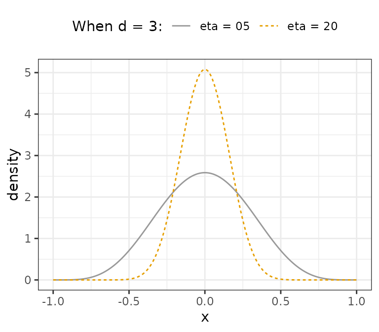
We see that larger values of lkj_shape can be used to
constrain interfactor correlations.
ml_par and sl_par
ml_par and sl_par are the prior mean and SD
for loadings which are assumed to be normally distributed. Note that
factors are assumed to be standardized.
rs_par
Residual standard deviation parameters are assumed to follow a
location-scale Student-t distribution with degrees of freedom 3
(unchangeable), location 0 (unchangeable) and scale
rs_par.
sc_par
All coefficients in minorbsem are assumed to be
standardized. These coefficients are assumed normal with mean 0
(changeable, see section on latent
regression below) and SD of sc_par.
Simple changes to default priors
Holzinger-Swineford example
This dataset is discussed in the CFA tutorial.
##         x1   x2    x3       x4   x5        x6       x7   x8       x9
## 1 3.333333 7.75 0.375 2.333333 5.75 1.2857143 3.391304 5.75 6.361111
## 2 5.333333 5.25 2.125 1.666667 3.00 1.2857143 3.782609 6.25 7.916667
## 3 4.500000 5.25 1.875 1.000000 1.75 0.4285714 3.260870 3.90 4.416667
## 4 5.333333 7.75 3.000 2.666667 4.50 2.4285714 3.000000 5.30 4.861111
## 5 4.833333 4.75 0.875 2.666667 4.00 2.5714286 3.695652 6.30 5.916667
## 6 5.333333 5.00 2.250 1.000000 3.00 0.8571429 4.347826 6.65 7.500000
The scale of data is important for setting priors on model
parameters. The default priors for models fit with
minorbsem are reasonable when variables have standard
deviations close to 1. For this reason, we first check the standard
deviations of the relevant variables for this analysis:
apply(item_data, 2, sd) # compute SD of each variable## x1 x2 x3 x4 x5 x6 x7 x8 x9
## 1.167432 1.177451 1.130979 1.164116 1.290472 1.095603 1.089534 1.012615 1.009152All variables have standard deviations close to 1, so we can move forward with the data as they are. Otherwise, we would recommend re-scaling the variables.1
syntax_basic <- "
Visual =~ x1 + x2 + x3
Verbal =~ x4 + x5 + x6
Speed =~ x7 + x8 + x9"
Let’s fit the model with modified priors:
priors_modified <- new_mbsempriors(lkj_shape = 10, sl_par = .75)
priors_modified
## An object of class "mbsempriors"
## Slot "lkj_shape":
## [1] 10
##
## Slot "ml_par":
## [1] 0
##
## Slot "sl_par":
## [1] 0.75
##
## Slot "rs_par":
## [1] 1
##
## Slot "rc_par":
## [1] 2
##
## Slot "sc_par":
## [1] 0.5
##
## Slot "rm_par":
## [1] 0.15We can fit make the call to the minorbsem() function and
obtain the data list passed to Stan instead of fitting the model by
setting ret_data_list = TRUE:
base_dl <- minorbsem(
  syntax_basic, item_data,
  priors = priors_modified, ret_data_list = TRUE
)
## Processing user input ...
base_dl$shape_phi_c # reflects the shape of interfactor correlation matrix## [1] 10
base_dl$load_est # reflects prior mean for loadings## Visual Verbal Speed
## x1 0 0 0
## x2 0 0 0
## x3 0 0 0
## x4 0 0 0
## x5 0 0 0
## x6 0 0 0
## x7 0 0 0
## x8 0 0 0
## x9 0 0 0
base_dl$load_se # reflects prior SD for loadings## Visual Verbal Speed
## x1 0.75 0.75 0.75
## x2 0.75 0.75 0.75
## x3 0.75 0.75 0.75
## x4 0.75 0.75 0.75
## x5 0.75 0.75 0.75
## x6 0.75 0.75 0.75
## x7 0.75 0.75 0.75
## x8 0.75 0.75 0.75
## x9 0.75 0.75 0.75
base_dl$loading_pattern # shows indices for non-zero loadings## Visual Verbal Speed
## x1 1 0 0
## x2 2 0 0
## x3 3 0 0
## x4 0 4 0
## x5 0 5 0
## x6 0 6 0
## x7 0 0 7
## x8 0 0 8
## x9 0 0 9We can either run the model with:
base_mod <- minorbsem(syntax_basic, item_data, priors = priors_modified)or
base_mod <- minorbsem(data_list = base_dl, priors = priors_modified)The results would be identical. Adding
priors = priors_modified is optional.2
Examples of priors on specific loadings and coefficients
Small variance prior on all cross-loadings
Following Muthén and Asparouhov (2012),
one can estimate all cross-loadings by placing small variance priors on
them. Note that minorbsem contains a cleaner approach to the same task
with models of the form:
minorbsem(..., simple_struc = FALSE). But we demonstrate
the small variance approach to show how to set specific priors on some
loadings.
syntax_cross <- paste(
  paste0("Visual =~ ", paste0("x", 1:9, collapse = " + ")),
  paste0("Verbal =~ ", paste0("x", 1:9, collapse = " + ")),
  paste0("Speed =~ ", paste0("x", 1:9, collapse = " + ")),
  sep = "\n"
)
writeLines(syntax_cross)
## Visual =~ x1 + x2 + x3 + x4 + x5 + x6 + x7 + x8 + x9
## Verbal =~ x1 + x2 + x3 + x4 + x5 + x6 + x7 + x8 + x9
## Speed =~ x1 + x2 + x3 + x4 + x5 + x6 + x7 + x8 + x9Then we call minorbsem() with
ret_data_list = TRUE to obtain the data list:
small_var_dl <- minorbsem(syntax_cross, item_data, ret_data_list = TRUE)## Processing user input ...Set all cross-loadings to have prior SDs of 0.1:
small_var_dl$load_se## Visual Verbal Speed
## x1 1 1 1
## x2 1 1 1
## x3 1 1 1
## x4 1 1 1
## x5 1 1 1
## x6 1 1 1
## x7 1 1 1
## x8 1 1 1
## x9 1 1 1
small_var_dl$load_se[4:9, 1] <- 0.1
small_var_dl$load_se[-c(4:6), 2] <- 0.1
small_var_dl$load_se[1:6, 3] <- 0.1
small_var_dl$load_se
## Visual Verbal Speed
## x1 1.0 0.1 0.1
## x2 1.0 0.1 0.1
## x3 1.0 0.1 0.1
## x4 0.1 1.0 0.1
## x5 0.1 1.0 0.1
## x6 0.1 1.0 0.1
## x7 0.1 0.1 1.0
## x8 0.1 0.1 1.0
## x9 0.1 0.1 1.0Before fitting the model, minorbsem automatically identifies an indicator per factor that it uses to align the factor in the right direction. Given that all indicators reflect all factors, we would need to identify these indicators manually:
small_var_dl$markers## [1] 1 1 1
small_var_dl$markers <- c(1, 4, 7) # for visual, verbal and speed respectivelyThen fit the model:
small_var_mod <- minorbsem(data_list = small_var_dl)## Parameter estimates (method = normal, sample size(s) = 301)
## from op to mean sd 5.000% 95.000% rhat ess_bulk
## ───────────────────────────────────────────────────────────────────────────────
## Goodness of fit
## ───────────────────────────────────────────────────────────────────────────────
## PPP 0.427 1.002 1847
## RMSE 0.027 0.013 0.008 0.049 1.001 540
## ───────────────────────────────────────────────────────────────────────────────
## Factor loadings
## ───────────────────────────────────────────────────────────────────────────────
## Visual =~ x1 0.752 0.116 0.570 0.950 1.000 1796
## Visual =~ x2 0.557 0.102 0.393 0.732 1.000 2515
## Visual =~ x3 0.752 0.107 0.575 0.928 1.000 1931
## Visual =~ x4 0.035 0.074 -0.087 0.153 1.002 2831
## Visual =~ x5 -0.067 0.080 -0.198 0.064 1.002 2438
## Visual =~ x6 0.067 0.073 -0.054 0.185 1.002 2854
## Visual =~ x7 -0.141 0.079 -0.271 -0.014 1.000 2196
## Visual =~ x8 0.007 0.081 -0.126 0.143 1.001 2318
## Visual =~ x9 0.215 0.072 0.099 0.329 1.000 2456
## Verbal =~ x1 0.124 0.081 -0.017 0.252 1.000 2479
## Verbal =~ x2 0.013 0.071 -0.109 0.129 1.000 3101
## Verbal =~ x3 -0.080 0.075 -0.203 0.046 1.001 2881
## Verbal =~ x4 0.979 0.078 0.856 1.109 1.001 2310
## Verbal =~ x5 1.141 0.086 1.004 1.286 1.000 2292
## Verbal =~ x6 0.886 0.073 0.773 1.008 1.001 2033
## Verbal =~ x7 0.026 0.073 -0.097 0.147 1.001 2427
## Verbal =~ x8 -0.036 0.074 -0.159 0.089 1.002 2860
## Verbal =~ x9 0.034 0.067 -0.077 0.143 1.001 2373
## Speed =~ x1 0.051 0.082 -0.085 0.182 1.002 2954
## Speed =~ x2 -0.052 0.074 -0.175 0.069 1.000 3306
## Speed =~ x3 0.041 0.078 -0.090 0.166 1.001 3077
## Speed =~ x4 0.001 0.070 -0.115 0.114 1.002 2838
## Speed =~ x5 0.008 0.076 -0.119 0.136 1.000 2797
## Speed =~ x6 0.001 0.068 -0.110 0.112 1.000 2823
## Speed =~ x7 0.731 0.099 0.569 0.899 1.000 1672
## Speed =~ x8 0.779 0.102 0.620 0.961 1.000 1628
## Speed =~ x9 0.539 0.085 0.402 0.679 1.001 2146
## ───────────────────────────────────────────────────────────────────────────────
## Inter-factor correlations
## ───────────────────────────────────────────────────────────────────────────────
## Verbal ~~ Visual 0.360 0.106 0.180 0.527 1.001 2200
## Speed ~~ Visual 0.323 0.130 0.096 0.522 1.000 2226
## Speed ~~ Verbal 0.239 0.117 0.037 0.422 1.001 1951
## ───────────────────────────────────────────────────────────────────────────────
## Residual variances
## ───────────────────────────────────────────────────────────────────────────────
## x1 ~~ x1 0.670 0.131 0.445 0.873 1.001 1861
## x2 ~~ x2 1.089 0.118 0.904 1.280 1.001 2892
## x3 ~~ x3 0.729 0.129 0.516 0.936 1.001 1854
## x4 ~~ x4 0.375 0.088 0.226 0.511 1.001 1759
## x5 ~~ x5 0.420 0.112 0.233 0.600 1.001 2068
## x6 ~~ x6 0.374 0.074 0.248 0.493 1.002 1890
## x7 ~~ x7 0.698 0.117 0.500 0.886 1.001 1532
## x8 ~~ x8 0.443 0.123 0.215 0.620 1.001 1250
## x9 ~~ x9 0.583 0.076 0.459 0.710 1.000 2648
## ───────────────────────────────────────────────────────────────────────────────
##
##
## Column names: from, op, to, mean, sd, 5%, 95%, rhat, ess_bulkPriors on specific coefficients
Consider the latent regression model:
syntax_reg <- "
Visual =~ x1 + x2 + x3 + x9
Verbal =~ x4 + x5 + x6
Speed =~ x7 + x8 + x9
Verbal ~ Visual + Speed"
Assume we believe the most likely estimate of the coefficient from visual to verbal is .5, we can change the prior mean for this coefficient to .5. We first retrieve the data list object.
reg_dl <- minorbsem(
  syntax_reg, item_data,
  ret_data_list = TRUE
)
## Processing user input ...
reg_dl$coef_pattern # coefficient pattern, note non-zero cells## Visual Verbal Speed
## Visual 0 0 0
## Verbal 1 0 2
## Speed 0 0 0
reg_dl$coef_est # default prior means## Visual Verbal Speed
## Visual 0 0 0
## Verbal 0 0 0
## Speed 0 0 0
reg_dl$coef_est["Verbal", "Visual"] <- .5
reg_dl$coef_est # updated
## Visual Verbal Speed
## Visual 0.0 0 0
## Verbal 0.5 0 0
## Speed 0.0 0 0
reg_dl$coef_se # default prior SDs## Visual Verbal Speed
## Visual 0.5 0.5 0.5
## Verbal 0.5 0.5 0.5
## Speed 0.5 0.5 0.5Then we fit the model with the updated data list:
reg_mod <- minorbsem(data_list = reg_dl)## Parameter estimates (method = normal, sample size(s) = 301)
## from op to mean sd 5.000% 95.000% rhat ess_bulk
## ──────────────────────────────────────────────────────────────────────────────
## Goodness of fit
## ──────────────────────────────────────────────────────────────────────────────
## PPP 0.383 1.001 1536
## RMSE 0.037 0.012 0.019 0.058 1.002 591
## ──────────────────────────────────────────────────────────────────────────────
## Regression coefficients (outcome ~ predictor)
## ──────────────────────────────────────────────────────────────────────────────
## Verbal ~ Visual 0.418 0.075 0.291 0.543 1.009 1520
## Verbal ~ Speed 0.080 0.079 -0.053 0.208 1.003 2212
## ──────────────────────────────────────────────────────────────────────────────
## R square
## ──────────────────────────────────────────────────────────────────────────────
## Visual ~~ Visual 0.000 0.000 0.000 0.000
## Verbal ~~ Verbal 0.208 0.058 0.119 0.310 1.006 1894
## Speed ~~ Speed 0.000 0.000 0.000 0.000
## ──────────────────────────────────────────────────────────────────────────────
## Factor loadings
## ──────────────────────────────────────────────────────────────────────────────
## Visual =~ x1 0.919 0.105 0.754 1.106 1.002 718
## Visual =~ x2 0.495 0.089 0.349 0.638 1.002 1936
## Visual =~ x3 0.646 0.088 0.500 0.792 1.002 1702
## Visual =~ x9 0.397 0.079 0.267 0.528 1.000 2152
## Verbal =~ x4 0.997 0.074 0.881 1.125 1.002 1598
## Verbal =~ x5 1.084 0.079 0.956 1.216 1.001 2344
## Verbal =~ x6 0.927 0.066 0.818 1.037 1.004 2247
## Speed =~ x9 0.443 0.089 0.304 0.595 1.001 1729
## Speed =~ x7 0.648 0.092 0.505 0.802 1.002 1525
## Speed =~ x8 0.845 0.103 0.680 1.017 1.004 1162
## ──────────────────────────────────────────────────────────────────────────────
## Inter-factor correlations
## ──────────────────────────────────────────────────────────────────────────────
## Verbal ~~ Visual 0.000 0.000 0.000 0.000
## Speed ~~ Visual 0.272 0.088 0.125 0.417 1.001 2880
## Speed ~~ Verbal 0.000 0.000 0.000 0.000
## ──────────────────────────────────────────────────────────────────────────────
## Residual variances
## ──────────────────────────────────────────────────────────────────────────────
## x1 ~~ x1 0.525 0.172 0.195 0.767 1.005 614
## x2 ~~ x2 1.144 0.113 0.967 1.338 1.001 2797
## x3 ~~ x3 0.859 0.108 0.687 1.040 1.001 1521
## x9 ~~ x9 0.580 0.081 0.450 0.710 1.000 2098
## x4 ~~ x4 0.357 0.106 0.175 0.526 1.000 1152
## x5 ~~ x5 0.493 0.119 0.297 0.689 1.001 1622
## x6 ~~ x6 0.348 0.090 0.202 0.492 1.004 1646
## x7 ~~ x7 0.773 0.116 0.581 0.952 1.002 1436
## x8 ~~ x8 0.319 0.158 0.028 0.566 1.005 960
## ──────────────────────────────────────────────────────────────────────────────
##
##
## Column names: from, op, to, mean, sd, 5%, 95%, rhat, ess_bulkWe also show results from the fit with default priors:
reg_def_priors <- minorbsem(syntax_reg, item_data)## Parameter estimates (method = normal, sample size(s) = 301)
## from op to mean sd 5.000% 95.000% rhat ess_bulk
## ──────────────────────────────────────────────────────────────────────────────
## Goodness of fit
## ──────────────────────────────────────────────────────────────────────────────
## PPP 0.406 1.000 1728
## RMSE 0.038 0.012 0.019 0.059 1.002 666
## ──────────────────────────────────────────────────────────────────────────────
## Regression coefficients (outcome ~ predictor)
## ──────────────────────────────────────────────────────────────────────────────
## Verbal ~ Visual 0.414 0.076 0.286 0.537 1.002 2628
## Verbal ~ Speed 0.082 0.080 -0.052 0.213 1.002 1891
## ──────────────────────────────────────────────────────────────────────────────
## R square
## ──────────────────────────────────────────────────────────────────────────────
## Visual ~~ Visual 0.000 0.000 0.000 0.000
## Verbal ~~ Verbal 0.206 0.058 0.115 0.305 1.000 3167
## Speed ~~ Speed 0.000 0.000 0.000 0.000
## ──────────────────────────────────────────────────────────────────────────────
## Factor loadings
## ──────────────────────────────────────────────────────────────────────────────
## Visual =~ x1 0.910 0.101 0.750 1.083 1.000 1795
## Visual =~ x2 0.496 0.089 0.354 0.641 1.002 2577
## Visual =~ x3 0.647 0.086 0.507 0.786 1.001 2525
## Visual =~ x9 0.400 0.080 0.266 0.532 1.001 2263
## Verbal =~ x4 0.994 0.074 0.875 1.119 1.001 1420
## Verbal =~ x5 1.084 0.079 0.956 1.213 1.000 1994
## Verbal =~ x6 0.927 0.068 0.822 1.039 1.001 1798
## Speed =~ x9 0.446 0.088 0.306 0.591 1.001 1403
## Speed =~ x7 0.650 0.096 0.500 0.816 1.001 1543
## Speed =~ x8 0.842 0.108 0.668 1.020 1.001 1151
## ──────────────────────────────────────────────────────────────────────────────
## Inter-factor correlations
## ──────────────────────────────────────────────────────────────────────────────
## Verbal ~~ Visual 0.000 0.000 0.000 0.000
## Speed ~~ Visual 0.270 0.087 0.126 0.416 1.001 2005
## Speed ~~ Verbal 0.000 0.000 0.000 0.000
## ──────────────────────────────────────────────────────────────────────────────
## Residual variances
## ──────────────────────────────────────────────────────────────────────────────
## x1 ~~ x1 0.538 0.161 0.244 0.777 1.000 1599
## x2 ~~ x2 1.142 0.110 0.972 1.327 1.000 2459
## x3 ~~ x3 0.860 0.105 0.689 1.030 1.001 2330
## x9 ~~ x9 0.575 0.084 0.436 0.709 1.001 2067
## x4 ~~ x4 0.361 0.105 0.180 0.524 1.003 1151
## x5 ~~ x5 0.490 0.127 0.283 0.695 1.000 1464
## x6 ~~ x6 0.348 0.089 0.194 0.487 1.000 1495
## x7 ~~ x7 0.767 0.120 0.569 0.956 1.001 1337
## x8 ~~ x8 0.324 0.163 0.032 0.580 1.000 995
## ──────────────────────────────────────────────────────────────────────────────
##
##
## Column names: from, op, to, mean, sd, 5%, 95%, rhat, ess_bulk