rccme

The goal of rccme is to produce regression calibrated scores for downstream regression models.

Installation

You can install the latest version of rccme with:

install.packages(
  'rccme',
  repos = c(
    'https://jamesuanhoro.r-universe.dev',
    'https://cloud.r-project.org'
  )
)

Example

We show how to approach the model below:

library(rccme)

library(lavaan) # for data source and measurement models

## This is lavaan 0.6-21
## lavaan is FREE software! Please report any bugs.

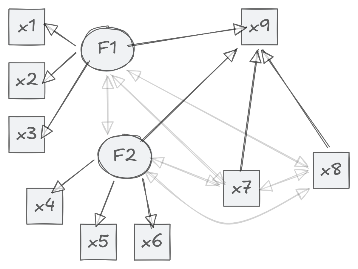
dat <- HolzingerSwineford1939[, paste0("x", 1:9)]

sem_fit <- sem(
  paste(
    "F1 =~ x1 + x2 + x3",
    "F2 =~ x4 + x5 + x6",
    "x9 ~ F1 + F2 + x7 + x8",
    "F1 + F2 ~~ x7 + x8",
    sep = "\n"
  ),
  dat,
  std.lv = TRUE
)

# two-step using factor analysis ----
cfa_f1 <- cfa("F1 =~ x1 + x2 + x3", dat, std.lv = TRUE)
cfa_f2 <- cfa("F2 =~ x4 + x5 + x6", dat, std.lv = TRUE)
score_f1 <- lavaan::lavPredict(cfa_f1, se = "standard")
score_f2 <- lavaan::lavPredict(cfa_f2, se = "standard")
se_f1 <- unname(attr(score_f1, "se")[[1]][, 1, drop = TRUE])
se_f2 <- unname(attr(score_f2, "se")[[1]][, 1, drop = TRUE])

# save factor scores
dat$f1 <- score_f1
dat$f2 <- score_f2

# calibrate factor scores
rc_fs <- rccme_calib_me(
  dat[, c("f1", "f2")],
  w_se_vec = c(se_f1, se_f2), z_mat = dat[, c("x7", "x8")]
)

# save calibrated factor scores
dat$f1_rc <- rc_fs[, 1]
dat$f2_rc <- rc_fs[, 2]

# two-step using sum-score ----
# compute standardised sum scores
dat$std_1 <- scale(rowMeans(dat[, c("x1", "x2", "x3")]))
dat$std_2 <- scale(rowMeans(dat[, c("x4", "x5", "x6")]))
# compute coefficient alpha
rel_1 <- psych::alpha(dat[, c("x1", "x2", "x3")])$total$raw_alpha

## Warning in response.frequencies(x, max = max): response.frequency has been
## deprecated and replaced with responseFrequecy.  Please fix your call

## Number of categories should be increased  in order to count frequencies.

rel_2 <- psych::alpha(dat[, c("x4", "x5", "x6")])$total$raw_alpha

## Warning in response.frequencies(x, max = max): response.frequency has been
## deprecated and replaced with responseFrequecy.  Please fix your call

## Number of categories should be increased  in order to count frequencies.

# calibrate sum scores
rc_ss <- rccme_calib_me(
  dat[, c("std_1", "std_2")],
  # Add `standard = TRUE` for standardised sum scores
  rel_vec = c(rel_1, rel_2), z_mat = dat[, c("x7", "x8")], standard = TRUE
)

# save calibrated sum scores
dat$std_1_rc <- rc_ss[, 1]
dat$std_2_rc <- rc_ss[, 2]

# model results ----
# sum-score without measurement error correction
fit_ss <- lm(x9 ~ std_1 + std_2 + x7 + x8, dat)
# sum-score without measurement error correction
fit_ss_rc <- lm(x9 ~ std_1_rc + std_2_rc + x7 + x8, dat)
# with standard factor scores
fit_fs <- lm(x9 ~ f1 + f2 + x7 + x8, dat)
# with calibrated factor scores
fit_fs_rc <- lm(x9 ~ f1_rc + f2_rc + x7 + x8, dat)

# SEM results
sem_fit |>
  parameterestimates() |>
  subset(op == "~")

##    lhs op rhs    est    se      z pvalue ci.lower ci.upper
## 7   x9  ~  F1  0.464 0.078  5.945  0.000    0.311    0.616
## 8   x9  ~  F2 -0.018 0.065 -0.285  0.776   -0.145    0.108
## 9   x9  ~  x7  0.191 0.046  4.138  0.000    0.101    0.282
## 10  x9  ~  x8  0.219 0.054  4.061  0.000    0.113    0.324

# Comparing the methods
modelsummary::modelsummary(
  list(
    "Sum score" = fit_ss,
    "Factor scores" = fit_fs,
    "Calibrated sum scores" = fit_ss_rc,
    "Calibrated factor scores" = fit_fs_rc
  ),
  # Rename calibrated variables:
  coef_rename = c(
    "std_1" = "F1", "std_2" = "F2",
    "std_1_rc" = "F1", "std_2_rc" = "F2",
    "f1" = "F1", "f2" = "F2",
    "f1_rc" = "F1", "f2_rc" = "F2"
  ),
  output = "markdown", gof_omit = "IC|R2|Log|F|RMSE|Obs", vcov = "HC4"
)

	Sum score	Factor scores	Calibrated sum scores	Calibrated factor scores
(Intercept)	3.123	3.157	3.324	3.346
	(0.239)	(0.238)	(0.244)	(0.244)
F1	0.321	0.395	0.450	0.427
	(0.052)	(0.063)	(0.074)	(0.070)
F2	0.074	0.085	-0.000	0.025
	(0.051)	(0.054)	(0.061)	(0.059)
x7	0.173	0.164	0.203	0.184
	(0.052)	(0.052)	(0.053)	(0.052)
x8	0.277	0.277	0.217	0.228
	(0.052)	(0.052)	(0.054)	(0.054)
Std.Errors	HC4	HC4	HC4	HC4